背景
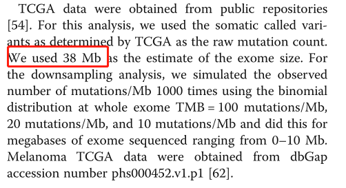
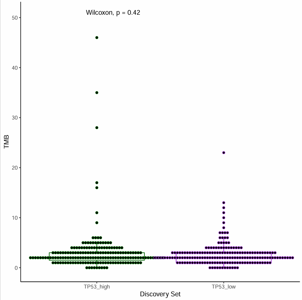
用TCGA的突变数据计算TMB,用某个基因的表达量来分组,画出带散点的box plot,计算p value。
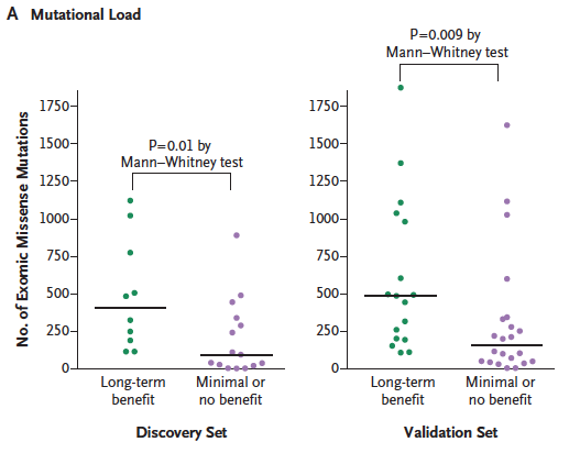
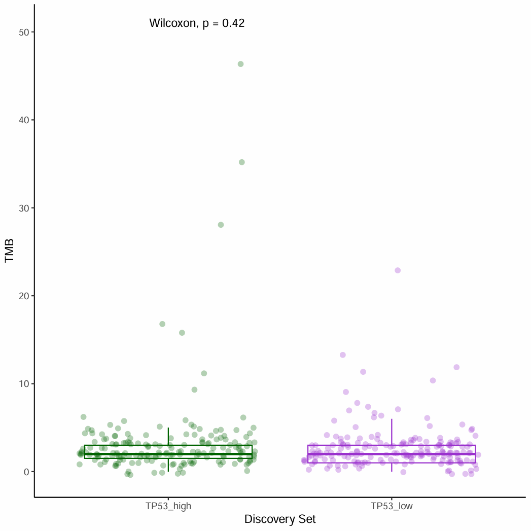
出自文章PMID: 25409260
应用场景
借助突变数据,把你的基因跟免疫治疗预后联系起来。
计算出每个sample的TMB,接下来就可以:
- 用某个基因表达量高低来分组,对比不同分组的TMB值。
- 用TMB值高低来分组,做生存分析。
输入数据预处理
如果你的数据已经保存成 easy_input_mut.csv和 easy_input_group.csv的格式,就可以跳过这步,直接进入“输入文件”。
从TCGA下载突变数据
TCGA已经给出了somatic mutation信息,因此,计算TMB非常简单方便。
此处以LIHC为例:
#source("https://bioconductor.org/biocLite.R")
#biocLite("TCGAbiolinks")
#biocLite("maftools")
require(TCGAbiolinks)
require(maftools)

#下载突变数据
# 下载 LIHC 突变数据
query <- GDCquery(
    project = "TCGA-LIHC",
    data.category = "Simple Nucleotide Variation",
    data.type = "Masked Somatic Mutation",
    workflow.type = "Aliquot Ensemble Somatic Variant Merging and Masking"
)
GDCdownload(query)
LIHC_mutect2 <- GDCprepare(query)

#确认是否都是somatic mutation
levels(factor(LIHC_mutect2$Mutation_Status))
没错,都是somatic mutation
接下来,有两种方法获得每个sample的variants数:
- 方法一:直接使用自带的variants.per.sample
#用maftools里的函数读取maf文件
var_maf <- read.maf(maf = LIHC_mutect2, isTCGA = T)
str(var_maf)

#并且已经统计好了每个sample里的variants数量
variants_per_sample <- [email protected]
dim(variants_per_sample) # 368 2
#保存到文件
write.csv(variants_per_sample, "easy_input_mut1.csv", quote = F, row.names = F)
- 方法二:自己计算每个sample的variants数量
在这个过程中可以删一下 silent 或其他你想删除的行
require(dplyr)

mutect.dataframe <- function(x){
  #删除Silent的行
  #cut_id <- x$Variant_Classification == "Silent"
  #x <- x[!cut_id,]
  somatic_sum <- x %>% group_by(Tumor_Sample_Barcode) %>% summarise(TCGA_sum = n())
}
variants_per_sample <- mutect.dataframe(LIHC_mutect2)
dim(variants_per_sample) # 371 2
head(variants_per_sample)

#保存到文件
write.csv(variants_per_sample, "easy_input_mut2.csv", quote = F, row.names = F)
对比两种方法获得的variants_per_sample:
require(stringr)

mut1 <- read.csv("easy_input_mut1.csv")
mut2 <- read.csv("easy_input_mut2.csv")
mut2$Tumor_Sample_Barcode <- str_sub(mut2$Tumor_Sample_Barcode,1, 12)
mut12 <- merge(mut1, mut2, by = "Tumor_Sample_Barcode")
colnames(mut12) <- c("Tumor_Sample_Barcode","mut1","mut2")
head(mut12)
cor(as.numeric(mut12$mut1),as.numeric(mut12$mut2)) # 0.9763697
从TCGA下载表达数据
如果你已经有表达数据,就可以跳过这步,直接进入“根据表达量给sample分组”
参考 https://bioinfoer.com/forum.php?mod=viewthread&tid=548&extra=page%3D1 整理表达数据
TCGAbiolinks:::getProjectSummary("TCGA-LIHC")
# 新版是STAR - Counts
library(data.table)
options(datatable.fread.datatable=FALSE)#保证fread返回数据框
expMatrix <- fread('./TCGA_LIHC_Tpm.txt')
rownames(expMatrix) <- exp$gene_name
expMatrix <- expMatrix[-1]
#只取肿瘤组织
group_list <- ifelse(substr(colnames(expMatrix),14,14)=='0','tumor','normal')
expMatrix_tumor <- expMatrix[,group_list=='tumor']
dim(expMatrix_tumor)# 28776 371
#保存一个基因的表达量,此处选取TP53
write.csv(expMatrix_tumor["TP53",], "easy_input_expr.csv", quote=F, row.names = T)
根据表达量给sample分组
easy_input_expr.csv,某个基因在各个sample里的表达量。
第一列是sample ID,与突变数据里的sample ID一致;第二列是基因的表达量。
require(stringr)

myGene <- read.csv("easy_input_expr.csv")
myGene <- t(myGene)
myGene <- as.data.frame(myGene)
myGene$rownames <- rownames(myGene)
myGene <- myGene[-1,]
myGene <- myGene[,c(2,1)]
colnames(myGene) <- c("Tumor_Sample_Barcode","Expr") #改列名
#保留barcode的前三个label
library(stringr)
myGene$Tumor_Sample_Barcode <- str_sub(myGene$Tumor_Sample_Barcode,1, 12)
head(myGene)

#用表达量中值分为两组
myGene$Expr_level <- ifelse(myGene$Expr > median(myGene$Expr),"TP53_high","TP53_low")
write.csv(myGene[,c(1,3)], "easy_input_group.csv", quote = F, row.names = F)
输入文件
包含两个输入文件:
- easy_input_mut*.csv,每个sample中的variants总数。
- easy_input_group.csv,样品分组。
library(stringr)

#突变
#myMut <- read.csv("easy_input_mut1.csv")
myMut <- read.csv("easy_input_mut2.csv")
colnames(myMut) <- c("Tumor_Sample_Barcode","Variants")
#保留barcode的前三个label
myMut$Tumor_Sample_Barcode <- str_sub(myMut$Tumor_Sample_Barcode,1, 12)
head(myMut)

#分组
myGroup <- read.csv("easy_input_group.csv")
head(myGroup)
 发表于 2025-6-4 10:50:56
|
查看: 1972|
回复: 2
发表于 2025-6-4 10:50:56
|
查看: 1972|
回复: 2 |Archiver|手机版|小黑屋|bioinfoer
( 萌ICP备20244422号 )
|Archiver|手机版|小黑屋|bioinfoer
( 萌ICP备20244422号 )